DFT – Trigonometric representation
This is the second tutorial in our ongoing series on time series spectral analysis. In this entry, we will continue our discussion on discrete Fourier Transform in Excel, its interpretation, and application in the time domain.
The DFT is basically a mathematical transformation and maybe a bit dry, but we hope that this tutorial will leave you with a deeper understanding and intuition through the use of NumXL functions and wizards.
Background
There have been several inquiries since the time we released our first entry on DFT, especially about using the DFT components to represent the input data set as the sum of the trigonometric sine-cosine functions. The inquiries were motivated by using this representation to interpolate intermediate values and possibly extrapolate (aka forecast) beyond the input data set.
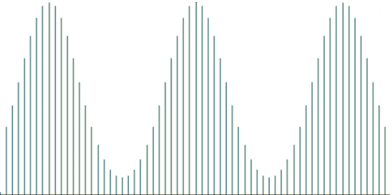
In principle, the DFT converts a discrete set of observations into a series of continuous trigonometric (i.e. sine and cosine) functions. So the original signal can be represented as:
Where:
- $x(t)$ is the value of the observation at time $t$.
- $t$ is the discrete time at which an observation was taken.
- $t \in \left \{ 0,1,2 \cdots N-1 \right \}$.
- $N$ is the number of observations in the input data set.
- $\omega = \frac{2\pi}{N}$ is the fundamental or principle frequency.
- $A_i\angle \phi_i$ is the amplitude and the phase of the i-th discrete Fourier component.
Analysis
Examining the Fourier transform’s components (i.e. amplitude and phase) of a finite series closer, we find the following observations:
- The amplitude series is symmetrical around the $N/2$ component.
- The phase of the $k$ component is the negative of the $N-k$ component.
In essence, we only need the 1st half of the DFT components to recover the original input data set. The original time is represented by the following components:
i \times t + \phi_i)\right)$$
Proof
t + \phi_i) +\sum_{i=N/2+1}^N A_i\times cos(\omega\times i \times t + \phi_i)
\right)$$
i \times t + \phi_i) +\sum_{i=N/2+1}^N A_{N-i}\times cos(\omega\times i \times
t – \phi_{N-i}) \right)$$
cos(\omega\times i \times t + \phi_i) +\sum_{i=1}^{N/2} A_i\times cos(\omega\times
(N-i) \times t – \phi_i) \right)$$
A_i\times cos(\omega\times i \times t + \phi_i) + A_i\times cos(\omega\times
(N-i) \times t – \phi_i) \right)$$
A_i\times cos(\omega\times i \times t + \phi_i) + A_i\times cos(2\pi\times t
-(\omega\times i \times t + \phi_i)) \right)$$
2\times \sum_{i=1}^{N/2} A_i\times cos(\omega\times i \times t + \phi_i)\right)$$
IMPORTANT: For an even-sized input data set, the last DFT component does not need to be multiplied by 2. So the cosine representation of the input data is expressed as follows:
i \times t + \phi_i)+ A_{N/2}\times cos(\omega\times \frac{N}{2} \times t + \phi_{N/2})\right)$$
i \times t + \phi_i)+ A_{N/2}\times cos(\pi \times t + \phi_{N/2})\right)$$
A_o + 2\times \sum_{i=1}^{N/2-1} A_i\times cos(\omega\times i \times t + \phi_i)+
A_{N/2}\times cos(\phi_{N/2})cos(\pi \times t)\right)$$
Conclusion
Using the discrete Fourier transform, we represent the discrete input data set as the sum of deterministic continuous trigonometric functions.
Dissimilar to the original data, which is defined at discrete time instances, the Fourier representation is continuous and thus defined at all-time values. Using this continuous representation, we can interpolate any values in this range (but not for extrapolation/forecast).
Files Examples
Please click the button below to download DFT trigonometric representation example.


