Volatility 101
This is the first entry in what will become an ongoing series on volatility modeling. In this paper, we will start with the definition and general dynamics of volatility in financial time series. Next, we will use historical data to develop a few methods to forecast volatility. These methods will pave the road to more advanced treatment in future issues.
Why should you care? Predicting volatility is crucial for many functions in financial markets. For a start, volatility is used by many for risk management (e.g. VaR), options pricing, asset allocation, and many other applications. Understanding volatility is vital for virtually all time series analysis.
For a data sample, we will use the S&P 500 daily returns between Jan 2002 and June 8, 2012. All examples are carried on in Excel using only NumXL functions.
By the end of this paper, we hope to leave you with an understanding of the different types of market volatility and develop an intuition for volatility dynamics.
Background
In finance, volatility is a measure for variation (i.e., risk) of the price of a financial instrument over time. Before we go into the types of volatilities, let’s take a step back and define it.
Volatility is commonly used to reference the standard deviation ($\sigma_T^2$) of the underlying distribution. An unbiased estimate of the population variance ($\sigma_T^2$ ) is defined as follows:
$$\hat \sigma_T^2=\frac{\sum_{i=1}^T (r_i-\bar r)^2}{T-1}$$
Where:
- $r_i$ is the holding period (e.g. daily, weekly, monthly, etc.) for returns.
The volatility (or standard deviation) is defined by a holding period, so weekly volatility is different than annual volatility.
Furthermore, the definition above calculates the average variance over the sample period. Assuming the excess returns (i.e. $r_i – \bar r$ ) are stationary (or weak-sense stationary), then $\sigma$ is a good forecast for future volatility. For a financial time series, do the stock’s returns exhibit time-invariant volatility? Let’s consider the S&P 500 daily returns example:
S&P 500 Application
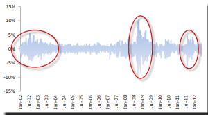
The daily log return of the S&P 500 Index exhibits common patterns that are well-documented in financial literature:
- Volatility Clusters – volatility may be high for a certain time period (red-circles) and low for other periods
- Volatility evolution – the volatility evolves over time in a continuous manner; i.e. volatility jumps are very rare.
- Volatility does not diverge to infinity– the volatility may go high (and stay high) in some time periods, but surely goes down to some steady-state value (long-run).
- Volatility does not go down to zero – the volatility may be low for a period of time, but it surely goes up to a steady-state level.
- Volatility reacts more to large negative returns than it does to similar positive ones.
In short, volatility does change over time, but only as a more stationary continuous mean-reverting process (Hint: ARMA process).
The main takeaway is that the volatility changes over time, so a forecast using historical volatility (which ignores volatility dynamics) may not be as robust or indicative for future ones.
Moving-window Standard Deviation
Using historical returns, we can compute the standard deviation using a sliding window (width h). This approach is an improvement over the historical one, but we are still making one implicit assumption:
“The observed volatility in the last time window is indicative for next-period volatility.”
What is the optimal size of the moving window?
In principle, the shorter the window is, the more responsive the moving standard deviation is to volatility changes; however, it can be very noisy too. On the other extreme, a larger window is less noisy, but it is slower to respond to changes in volatility. With that in mind, what is the optimal value that can give us a good volatility forecast?
To answer this question, we need to develop a utility (or loss) function that we opt to maximize (or minimize) by altering the window size (h). Let’s formulate the problem:
$$\hat \sigma_t^2=\frac{\sum_{i=1}^h (r_{t-i}-\bar r_t)^2}{h-1}$$ $$\bar r_t=\textrm{MA}=\frac{\sum_{i=1}^h r_{t-i}}{h}$$
Where:
- $\sigma_t$ is the volatility forecast using prior information $\{r_{t-1},r_{t-2},\cdots,r_{t-h}\}$
- $r_t$ is the moving average for the same window
To gauge how bad our forecast is, we will use the root mean squared error (RMSE) as our loss function (i.e. the smaller the RMSE the better).
$$\mathrm{RMSE}=\sqrt\frac{\sum_{i=h}^{T}(\hat\sigma_t^2-r_t^2)^2}{T-h}$$
Where:
- $r_t^2$ is used in place of the actual (realized) volatility
- $(T-h)$ is the number of volatility forecasts available
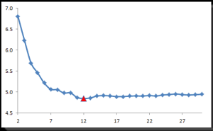
Next, we’ll compute the RMSE for different window sizes between 2 and 30 days, evaluate the RMSE, and pick the one with the minimal value.
In the plot above, a window size of 12-day has the lowest RMSE, after which the RMSE stabilizes. The takeaway here is that the window size should not be less than 10 days for a good forecast.
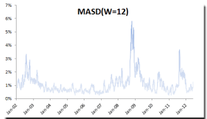
Using moving standard deviation with a window size = 12, let’s plot the volatility forecast:
The moving standard deviation method is an improvement over plain historical volatility as it responds to changes in volatility over time, but it gives all observations (within its window) equal weights.
Weighted Moving-Window Standard Deviation
A natural extension to the moving average is to assign weights to observations in the window; recent observations are given higher weight factors (similar to weighted-moving average) than later ones.
In practice, exponential weighted volatility (EWMA) is the most commonly used.
Exponential-Weighted Moving Average (EWMA)
In 1992, JP Morgan launched their RiskMetrics methodology to the marketplace, making their substantive research and analysis internally available to market participants. EWMA is part of RiskMetrics methodology.
$$\hat \sigma_t^2 = \lambda \times \hat \sigma_{t-1}^2 + (1-\lambda)\times r_{t-1}^2$$
Where:
- $\lambda$ is the exponential smoothing parameter $(0 \leq \lambda \leq 1)$
let’s expand the EWMA definition a bit more:
$$\hat \sigma_t^2 = \lambda \times \hat \sigma_{t-1}^2 + (1-\lambda)\times r_{t-1}^2 = \lambda (\lambda \times \hat \sigma_{t-2}^2 + (1-\lambda)\times r_{t-2}^2) +(1-\lambda)\times r_{t-1}^2$$ $$\hat \sigma_t^2 = \lambda^2 \hat \sigma_{t-2}^2 + (1-\lambda)(r_{t-1}^2+\lambda r_{t-2}^2) = \lambda^3 \hat \sigma_{t-3}^2+(1-\lambda)(r_{t-1}^2+\lambda r_{t-2}^2 + \lambda^2 r_{t-3}^2)$$ $$\hat \sigma_t^2 = \lambda^k \hat \sigma_{t-k}^2+(1-\lambda)\sum_{i=1}^{k}\lambda^{i-1}\times r_{t-i}^2$$
The EWMA has a few favorable properties:
- Weights sum up to one (1).
$$(1-\lambda)\sum_{i=1}^{\infty}\lambda^{i-1}=(1-\lambda)\sum_{i=0}^{\infty}\lambda^{i}=\frac{1-\lambda}{1-\lambda}=1$$ - Higher weights are given to recent observations, declining exponentially afterward
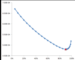
In RiskMetrics, JP Morgan uses $\lambda=0.94$ for almost everything, but let’s compute an optimal value of $\lambda$ using the same methodology in the MASD earlier.
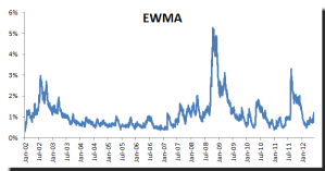
The optimal value for $\lambda$ using the S&P 500 daily returns is found at 0.90, which is very close from the rule-of-thumb of 0.94 (see the graph above).
Let’s plot the daily volatility forecast using the EWMA and $\lambda=0.90$.
Comparing the EWMA volatility with the ones we obtained in the moving-window standard deviation method, we see that they are pretty close. However, the EWMA method gave us a slightly lower RMSE and was much easier to calculate.
The EWMA is an improvement over moving average (i.e. simplicity), but it also suffers from a few drawbacks, including the fact that it is Symmetric; that is, large negative returns have the same effect as large positive ones. As a result, it does not capture the volatility dynamics, but it merely smooths the squared time series.
In fact, the EWMA is actually Brown’s simple exponential smoothing function for the squared returns, so the multi-step forecast is pretty flat (as it is in Brown’s formula).
$$\hat \sigma_{t+1}^2 = \lambda \times \hat \sigma_{t}^2 + (1-\lambda)\times r_{t}^2$$ $$\hat \sigma_{t+2}^2 = \lambda \times \hat \sigma_{t+1}^2 + (1-\lambda)\times \hat \sigma_{t+1}^2 = \hat \sigma_{t+1}^2$$ $$\hat \sigma_{t+k}^2=\hat \sigma_{t+1}^2$$
Conclusion
In this paper, we started by discussing the general patterns found in financial time series (e.g. clustering, reversion to the mean, asymmetrical reaction to positive and negative returns), and followed that by introducing two methods for estimating volatility using historical data: moving standard deviation and exponential weighted volatility (EWMA).
To compare the goodness of volatility forecast of each method, we leveraged the root-mean-squared error (RMSE) between the squared daily returns and estimated variance. Using RMSE as a loss-function, we computed the optimal values for the moving window size and the EWMA smoothing parameter.
Furthermore, we compared the RMSE value of each method and found that EWMA slightly fits; not to mention it was easier to calculate.
Finally, neither method captures any of the dynamics of the volatility process; they are at best smoothing functions which give a good estimate over a very short horizon.
Appendix
For estimating stock volatility using historical data, some academics proposed an alternative formula to replace the standard deviation calculation by leveraging daily open-close, daily hi-lo information to improve the estimate. Here’s a list of a few of them:
- Parkinson – named after physicist Michael Parkinson, this method uses only the daily HI-LO to estimate next-day volatility.
- Garman-Klass – developed by Graman and Klass, it uses the high, low, and close prices to estimate volatility.
- Yang Zhang – an extension of the Garman-Klass estimate, it uses open, hi, lo, and close prices to estimate future volatility.


